


What is Linear Programming?
Linear programming (LP) is a method of optimisation. It is used when we want to maximise or minimise a quantity (such as profit, cost, or time) while working under certain constraints (such as limited resources, time, or materials).
In LP:
- The unknowns are called decision variables.
- The formula to optimise is called the objective function.
- The limits or rules are expressed as linear inequalities or equations called constraints.
The solution is the set of values for the decision variables that gives the best result while satisfying all constraints.
Why is Linear Programming Important?
Linear programming is important because it helps us make the best possible decision when resources are limited. It is widely used in:
- Business & Economics – to maximise profit or minimise costs.
- Manufacturing – to decide the best mix of products with limited resources.
- Transportation & Logistics – to minimise delivery costs or times.
- Energy & Engineering – to optimise resource allocation and system design.
In short, LP provides a systematic way to achieve efficiency and avoid waste.
1. Decision Variables – the unknowns we want to solve for (e.g. number of products).
2. Objective Function – the quantity to maximise or minimise.
3. Constraints – the rules or limits written as linear inequalities/equations.
4. Non-Negativity – variables must be greater than or equal to zero.
5. Feasible Region – the set of all possible solutions that satisfy every constraint.
🔹 Steps for Solving Linear Programming Problems
To solve a linear programming problem effectively, follow these key steps. These are the standard methods used at A-Level for two-variable problems that can be solved graphically.
1. Define the decision variables
Start by identifying what the problem is asking you to find. Usually, this involves quantities such as the number of units produced or hours allocated. Assign variables (typically x and y) to represent these unknowns.
Example: Let x be the number of tables produced, and y the number of chairs.
2. Write the objective function
The objective function is the formula you want to maximise or minimise—often profit, cost, or time. It will usually be a linear equation in terms of x and y.
Example: Maximise profit

3. Formulate the constraints
Write out the inequalities based on the problem's limitations—such as time, materials, or budget. These are the conditions the solution must satisfy. Also, include non-negativity constraints x≥0x \geq 0x≥0 and y≥0y \geq 0y≥0, since negative quantities often don’t make sense in real-world scenarios.
Example:
 (material limit)
 (labour limit)
4. Draw the feasible region
On graph paper or using graphing software, plot each constraint as a straight line and shade the region that satisfies all the inequalities. The feasible region is the area where all constraints overlap.
5. Identify the corner (vertex) points
The maximum or minimum value of the objective function will occur at one of the corner points (vertices) of the feasible region. Find the coordinates of each vertex—either by observation, solving equations simultaneously, or using intersection points.
6. Evaluate the objective function at each vertex
Substitute the coordinates of each vertex into the objective function. Compare the results to determine the maximum or minimum value, depending on what the question asks.
Example:
Test
at each vertex and identify the one that gives the highest profit.
7. State the final solution clearly
Write out the optimal values of x and y, and what they represent in context (e.g. number of items to produce), along with the maximum or minimum value of the objective function.
These concepts combine algebra, graphical representation, and logical reasoning—making linear programming a valuable tool not only in mathematics exams but also in solving practical problems in business, science, and industry.
In the exercises below, you’ll find word problems typical of A-Level assessments, each followed by a fully worked solution. These will help you understand how to model real-life situations mathematically, interpret inequalities, and apply systematic methods to find optimal results.
Worked Example: Bakery Problem
Problem:
A bakery makes caramel cookies (x) and chocolate chip cookies (y):
- At least 80 caramel and 120 chocolate chip must be made daily.
- At most 120 caramel and 140 chocolate chip can be made.
- At least 240 cookies in total must be produced daily.
- Profit: $1 per caramel, $0.88 per chocolate chip.
How many of each cookie should be made to maximise profit?
Step 1 – Decision Variables
x = caramel cookies
y = chocolate chip cookies
Step 2 – Objective function
P = 1x + 0.88y
Step 3 – Constraints
x ≥ 80
x ≤ 120
y ≥ 120
y ≤ 140
x + y ≥ 240
x, y ≥ 0
Step 4 – Draw the graph

Step 5 – Identify corner points
(100,140), (120,120), (120,140)
Step 6 – Evaluate
P(100,140)=223.2
P(120,120)=225.6
P(120,140)=243.2
Step 7 – Best solution
Maximum profit = $243.20, at 120 caramel and 140 chocolate chip cookies.
Practice Examples (with Solutions)
A shop makes chairs (x) and tables (y). Calculate the maximum profit given the below constraints:
Chair: 2 hrs carpentry, 3 hrs painting.
Table: 3 hrs carpentry, 2 hrs painting.
Max: 60 carpentry hrs, 48 painting hrs.
Profit: $30 per chair, $40 per table.
Step 1 – Define variables
x = number of chairs
y = number of tables
Step 2 – Objective function
Maximise: P = 30x + 40y
Step 3 – Constraints
2x + 3y ≤ 60 (carpentry)
3x + 2y ≤ 48 (painting)
x, y ≥ 0
Step 4 – Draw graph
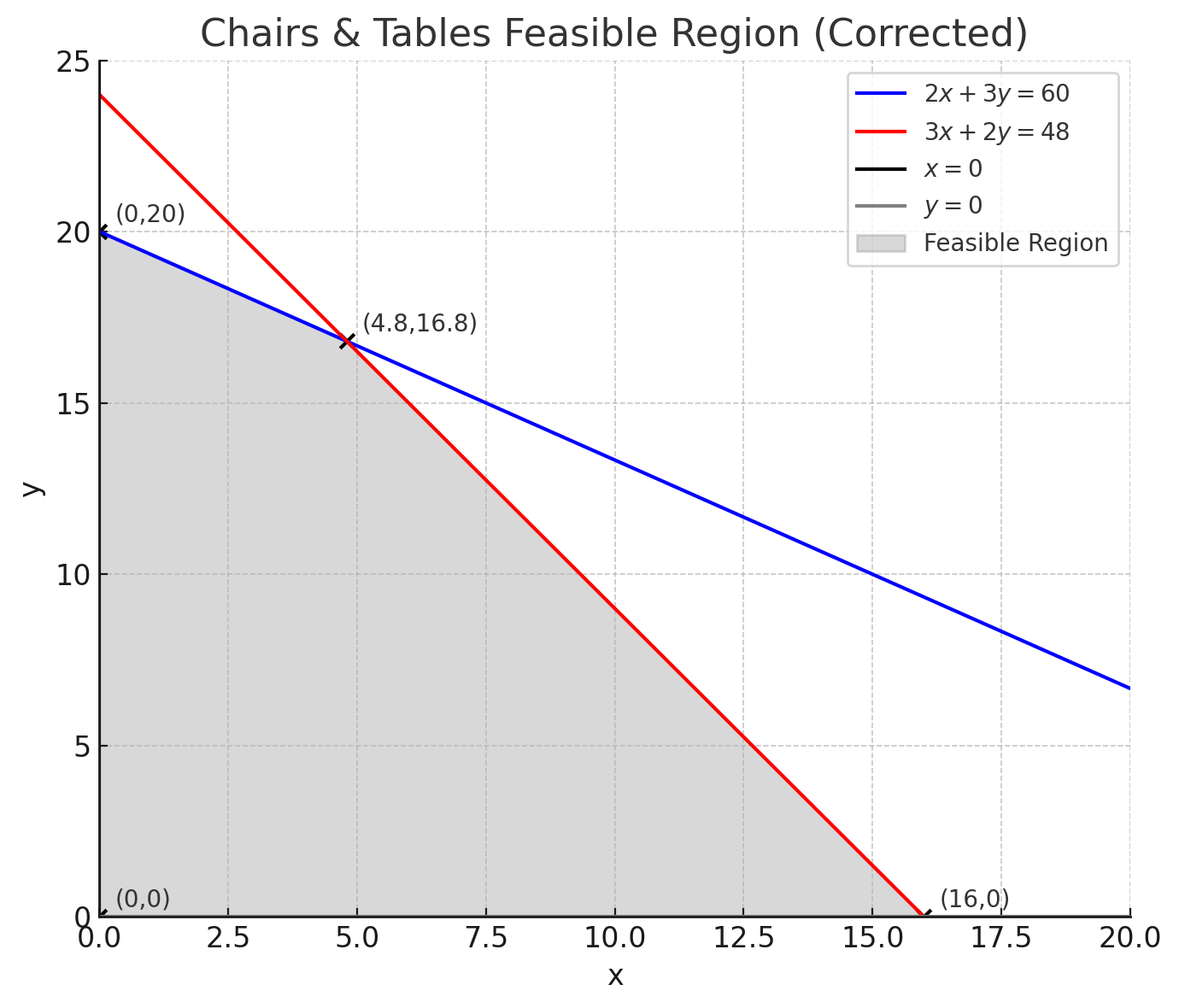
Step 5 – Corner points(0,0), (16,0), (0,20)
Intersection of 2x + 3y = 60 and 3x + 2y = 48 → (4.8,16.8). However, we cannot have fractional numbers of chairs and tables so this vertex can be discarded.
Step 6 – Evaluate objective function
P(0,0) = 0
P(16,0) = 480
P(0,20) = 800
Step 7 – Conclusion
Maximum profit = $800 at (x,y) = (0,20)
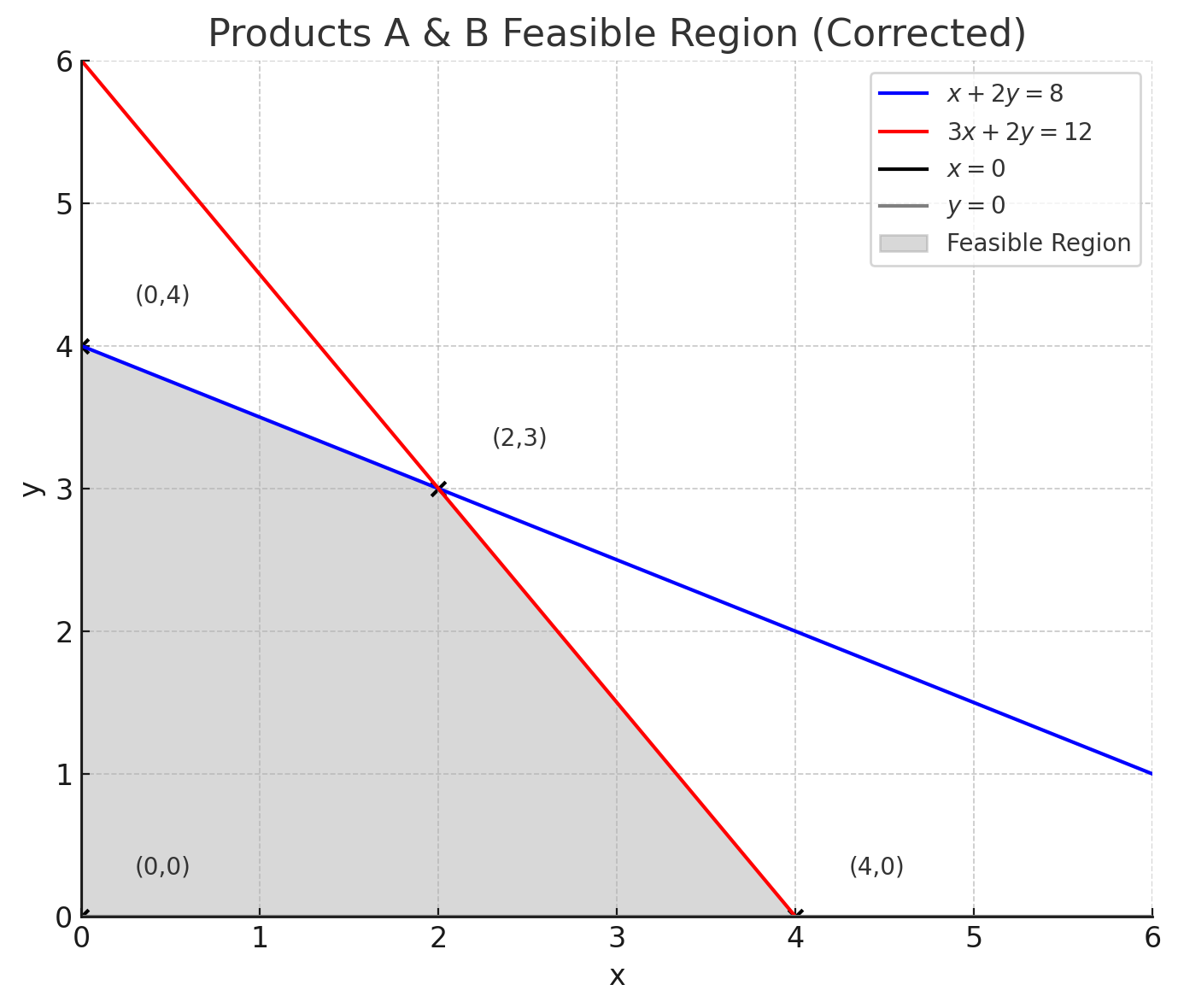
A factory makes products A (x) and B (y). Calculate the maximum profit given the below constraints:
A: 1 unit raw material, 3 hrs labour
B: 2 units raw material, 2 hrs labour
Available: 8 raw units, 12 labour hrs
Profit: $20 per A, $30 per B
Step 1 – Define variables
x = number of A
y = number of B
Step 2 – Objective function
Maximise: P = 20x + 30y
Step 3 – Constraints
x + 2y ≤ 8 (raw materials)
3x + 2y ≤ 12 (labour)
x, y ≥ 0
Step 4 – Draw graph
Step 5 – Corner points
(0,0), (4,0), (0,4)
Intersection of x + 2y = 8 and 3x + 2y = 12 → (2,3)
Step 6 – Evaluate objective function
P(0,0) = 0
P(4,0) = 80
P(0,4) = 120
P(2,3) = 130
Step 7 – Conclusion
Maximum profit = $130 at (x,y) = (2,3).
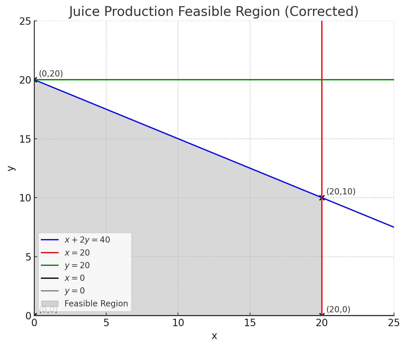
A company makes orange juice (x) and apple juice (y). Calculate the maximum profit given the below constraints:
Orange juice: 2 oranges + 1 hr per litre
Apple juice: 3 apples + 2 hrs per litre
Available: 40 oranges, 60 apples, 40 hours
Profit: $4 per orange juice, $5 per apple juice
Step 1 – Define variables
x = litres of orange juice
y = litres of apple juice
Step 2 – Objective function
Maximise:
P = 4x + 5y
Step 3 – Constraints
2x ≤ 40 → x ≤ 20 (oranges)
3y ≤ 60 → y ≤ 20 (apples)
x + 2y ≤ 40 (time)
x, y ≥ 0
Step 4 –Draw Graph
Step 5 – Corner points
(0,0), (20,0), (0,20), (20,10)
Step 6 – Evaluate objective function
P(0,0) = 0
P(20,0) = 80
P(0,20) = 100
P(20,10) = 130
Step 7 – Conclusion
Maximum profit = $130 at (x,y) = (20,10).
Get more practice with our linear programming practice questions.
Summarise with AI:
Did you like this article? Rate it!


Nice work but I get confused on how certain things work and I wish I can get someone to explain it to me better
Thanks for your feedback! Linear programming can definitely be tricky at first, so you’re not alone. If you’d like a clearer explanation, working through examples with a tutor or getting step-by-step guidance can really help. Feel free to let us know what you find most confusing — we’re happy to help point you in the right direction. 😊
I hope that there are people that need more problem solution
Thanks for your comment! We’re glad you found the solutions helpful — and we agree, more worked examples can make a big difference when learning linear programming. We’ll keep that in mind for future updates. 😊
GOOD PRESENTATION. DO YOU HAVE ONE ON COORDINATE GEOMETRY?
Thanks so much! I’m really glad you liked the presentation. Yes — we actually do have a great set of resources on coordinate geometry. You can find them here:
👉 https://www.superprof.co.uk/resources/academic/maths/geometry/
The language in the third question is confusing. “Offer A is a package of one shirt and a couple of pants which will sell for “. A couple of pants indicate 2 pants instead of a single pair of pant, it could’ve been renamed as a pair of pant. Couple of pant”s” means plural. Please change the language. From my understanding, the offer A consisted of 1 shirt and 2 pants, but in the solution, they have considered one shirt and one pant.
Thank you for your feedback! You’re absolutely right — the wording around “a couple of pants” was confusing. The problem has now been updated to clearly state that Offer A includes one shirt and one pair of pants, which aligns with the solution provided. We appreciate you taking the time to point this out and helping us improve the clarity of the question.
Hi there, thanks for your comment and for taking the time to share your calculation!