Hypothesis Testing Problems

What is a Hypothesis?

Ever make bets with your family and friends about sports, singing or dancing competitions? You can think of these bets as a hypothesis. A hypothesis is defined as a proposed explanation for an event based on previous facts. A hypothesis is little more than an educated guess. This is why, when you make a bet on a winning singer in a talent competition, you are making a hypothesis. You are using previous information in the form of past performances to propose an explanation for the future. Take a look at the table below for an example of hypotheses in various fields.

Field	Hypothesis
Psychology	Twins have the same IQ
Biology	Fertilizer increases average height growth for plants
Political Science	Countries that received a loan are better off now than those who didn’t

What is Hypothesis Testing?

Now that you understand the definition of a hypothesis, you can start to delve into the basics of hypothesis testing. Hypothesis is exactly what it sounds like - you conduct a hypothesis test in order to test whether or not your hypothesis is probable. Using the probabilities in your data, you can determine how likely your hypothesis is true most of the time or simply the result of chance. Hypotheses have a special notation, which are introduced below.

	Null hypothesis
	Alternative hypothesis
	Population mean
	Population standard deviation
	Sample mean
	Sample SD

Let’s focus on the first two lines - the rest will be explained further. The null and alternative hypotheses are the two types of hypotheses you can make about your data. The definitions of each are summarized in the table below.

	States that a parameter is equal to, less or greater than, or different from a hypothesized value
	States that a parameter is not equal to, less or greater, or different from a hypothesized value

Hypothesis tests can be conducted by finding the probability distribution of your data. The frequency distribution of your data set is simply the frequency at which each value in the data set occurs. Probability distributions, on the other hand, use the mean and standard deviation of your data set to produce the likelihood of certain values occurring.

Types of Hypothesis Testing

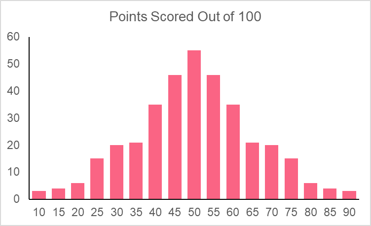
Building off of the previous section, you now know that we can make hypothesis tests based off of a data set’s probability distribution. In fact, most of the time you can make hypothesis tests without the entire data set and simply use the mean and standard deviation information. Hypothesis tests can be made using probability distributions because you can see whether or not your hypothesized value is likely to occur. Recall, however, that there are many types of distributions. Take a look at the table below, which summarizes each hypothesis test, their required distributions and their test parameters.

Test Type	Distribution	Test Parameters
Z-test	Normal	Mean
T-test	Student-t	Mean
ANOVA	F distribution	Means
Chi-Square	Chi-squared distribution	Association between two categorical variables

As you can see, while the first three are used for the comparison of means, the last test is used to compare the association between two categorical variables. Each hypothesis test uses these basic principles.

Element	Example	Description
Hypothesis with hypothesized value		The here is that the population mean is greater than 45
Test value	45	This is used as a benchmark to test how likely a mean of 45 is given the population mean and SD
Confidence interval		At the 95% confidence level (1-0.95 = 0.05), we can be certain that our test gets the true answer 95% of the time
Test statistic		The test statistic gives you the standardized value of your test value on your test distribution
P-value		The p-value is the calculated probability of your value occuring

In hypothesis testing, the following rules are used to either reject or accept the hypothesis given a

of 0.05. Keep in mind that if you were to have an

of 0.1, you’re results would be given with 90% confidence and the example above, with a p-value of 0.06, would reject

.

P-value <0.05	Region of rejection	Reject
P-value > 0.05	Region of acceptance	Fail to reject

Type 1 and Type 2 Error

To understand type 1 and type 2 error, let’s take a closer look at the confidence level. Take as an example a scenario in which you are conducting an experiment on average plant growth in one year as a result of a specific fertilizer. Recall that a population is the thing or idea that you want to study - here, it would be the plant we are studying. Because it is impossible for us to test our hypothesis on all of the plants in the world, we take samples in order to make estimates about the population. Let’s assume we’ve taken 100 different samples from this plant population. A confidence level is defined as the percentage of all possible samples that we can expect to include the true population parameter. A 95% confidence level would therefore be the same as saying that we expect 95% of all 100 samples to include the true population parameter. A confidence level can be set at a ton of different values. In fact, the DNA tests that people take nowadays to find out where their ancestors come from include varying confidence levels you can set. The table below summarizes common confidence levels with their corresponding

, or alpha, value.

Confidence Level	Alpha
99
95
90
85
75

Type 1 and 2 errors occur when we reject or accept our null hypothesis when, in reality, we shouldn’t have. This happens because, while statistics is powerful, there is a certain chance that you may be wrong. The table below summarizes these types of errors.

	Accept	Reject
In reality, is actually true	Correct: is true and statistical test accepts	Incorrect: Type 1 error - is true and statistical test rejects
In reality, is actually false	Incorrect: Type 2 error - is false and statistical test accepts	Correct: is false and statistical test rejects

 

Now that you’re familiar with hypothesis testing, let’s look at an example: The mean population IQ for adults is 100 with an SD of 15. You want to see whether those born prematurely have a lower IQ. To test this, you attain a sample of the IQ’s adults that were born prematurely with a sample mean of 95. Your hypothesis is that prematurely born people do not have lower IQs. Because we know the population mean and standard deviation, as well as the distribution (IQ’s are generally normally distributed), we can use a z-test.

Null Hypothesis	: IQ of 95 or above is normal
Alternative Hypothesis	: IQ of 95 is not normal

First, we find the z-score Next, we find the z-score on a z-table for negative values.

Z	0.00	0.01	0.02	0.03
0.2	0.42074	0.41683	0.41294	0.40905
0.3	0.38209	0.37828	0.37448	0.37070

With a p-value of 0.3707, we the fail to reject the null hypothesis.

Type 1 Error Example

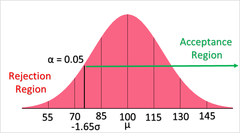
In the example above, you can see that we have chosen our confidence level to be at 95%. This gives us an alpha of 0.05. As explained above, a type 1 error occurs when our statistical test rejects the null hypothesis when, in reality, the null hypothesis is true. The main question is, how do we know when a type 1 error has occurred? The only way we could know for certain would be if we had all population values, which we don’t. Luckily, we can use the same logic as we do for the confidence level. If we are 95% certain of something occurring, this means that the probability that this thing really didn’t occur as the tail end of our rejection region. Therefore, the type 1 error is calculated simply as the 1 minus the probability that our hypothesis occurred, which is simply our p-value 0.3707.