The classic OLS assumptions make it possible for any least squares regression to be valid. Without these assumptions, the results of a least squares regression cannot be taken seriously. Try to test your knowledge on the OLS assumptions by answering the problem below. If you find that you’re having trouble answering or are encountering these concepts for the first time, take a read through this guide first.






Problem 6
You are given the following dataset and multiple regression model that explores the relationship between car sales blood pressure, weight, height and age. You’d like to conduct a multiple regression analysis but first want to check through the 6 OLS assumptions. Through the use of graphs and statistics, do you think this model passes each assumption? Explain why or why not.
| Blood Pressure | Weight | Height | Age |
| 105 | 75 | 172 | 19 |
| 106 | 80 | 175 | 18 |
| 108 | 89 | 170 | 20 |
| 110 | 90 | 174 | 20 |
| 113 | 93 | 178 | 21 |
| 115 | 95 | 179 | 22 |
| 118 | 96 | 180 | 24 |
| 119 | 99 | 183 | 25 |
| 120 | 101 | 185 | 29 |
| 122 | 102 | 188 | 30 |
OLS
Recall that ordinary least squares, or OLS, is a regression model that has the least squared errors. These population errors are estimated by the sample statistics called “residuals.” The most accurate regression line is one that reduces the space between the observed y values in the data and the estimated y values.
| 1 |  | OLS estimated regression equation |
| 2 |  | OLS equation rearranged to get residual formula |
| 3 |  | Residual is the difference between the observed and predicted value |
| 4 |  | Residuals are squared to counteract negative residuals |
OLS Assumptions
There are some assumptions that all linear models should pass in order to be taken seriously. These classical linear regression models, or CLRM assumptions, make up the Gauss-Markov theorem. This theorem states that when a model passes the six assumptions, the model has the best, linear, unbiased estimates, or BLUE. Check out the assumptions below.
| # | Assumption | Description |
| 1 | 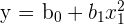 | Linear in parameters |
| 2 |  are random sample are random sample | If each individual in the same population is equally likely to be picked for the sample |
| 3 | 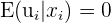 | Zero conditional mean of the error term |
| 4 | Weak correlation between  | No perfect collinearity |
| 5 |  | Homoskedasticity |
| 6 |  | No autocorrelation |
CLRM Assumption 1
The first assumption states that a regression model should be linear in parameters. Keep in mind that there is a difference between a model’s parameters and it’s variables.
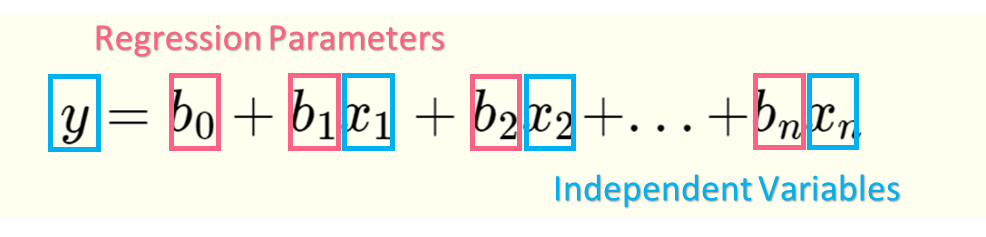
These parameters are called regression coefficients, which are estimated using each sample. Our independent variables, on the other hand, are represented by the y and . The model's parameters can only be linear, however the model's variables can be non-linear. To check this assumption, simply check the parameters.
| Linear in Parameters | Not Linear in Parameters |
 |  |
CLRM Assumption 2
This assumption states that the sample must be a random sample. This means that the sample is drawn from the same population where each sampled individual or value has an equal probability of being chosen. This also means that the sampled values are independent of each other.
To check this assumption, you simply have to find out the sampling methodology behind the data if you were not the one who took the sample. Check out the difference between sampling methodologies below.
| Random Samples | Non-random samples |
| SRS (Simple Random Sample) | Quota, Voluntary, Expert, or Convenience Sampling |
CLRM Assumption 3
The third assumption deals with the error term. This assumption states that the expected value, or mean, of the error term given  has to be zero. In other words, the x values cannot be correlated with the residual values. When the error term is correlated to any independent variables, this is called endogeneity.
Another term for endogeneity is omitted variable bias, where a crucial independent variable is omitted from your model. This crucial variable is then included in the error term, which, because it is correlated with the dependent variable, causes the error term to be correlated with the dependent variable.
You can check endogeneity with the Durbin-Wu-Hausman (DWH) test on any statistical program.
| No endogeneity | P-value < 0.05 | Endogeneity |
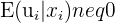 | Endogeneity | P-value > 0.05 | No endogeneity |
CLRM Assumption 4
The next assumption deals with collinearity. Perfect collinearity occurs when there is an exact linear relationship between two variables. Perfect collinearity can happen for many reasons, summarized below.
| One variable is a multiple of another variable | One explanatory variable (EV)  is in feet and another EV is in feet and another EV  is in meters is in meters |
| One variable is a linear combination of the others | is questions answered right, is answered wrong and  left unanswered, then total points = + + left unanswered, then total points = + + |
| One variable is a transformation of the other | is price and is the logarithm of price |
This can be checked with a correlation matrix, which lists all variables and their correlations.
| Height | Weight | Heartbeat Rate | |
| Height | 1 | 0.96 | 0.61 |
| Weight | 0.96 | 1 | 0.72 |
| Heartbeat Rate | 0.61 | 0.72 | 1 |
CLRM Assumption 5
The fourth assumption states that there should be no heteroskedasticity, meaning the variance shouldn’t have a pattern.

The above graph represents a heteroscedastic data set, where the pattern is that as the x value increases, the variance increases. As the x-value decreases, the variance decreases. Below are several ways to test for homoscedasticity.
| Residuals v Predicted Values Plot | Levene Test | Rule of thumb | |
| Homoscedastic | Null plot - no pattern | P-value > 0.05 | Largest variance is less than 3 to 5 times the smallest variance |
CLRM Assumption 6
The sixth assumption states there shouldn’t be any autocorrelation, or serial correlation. Meaning, different error terms cannot be correlated. Take the graph below as an example.
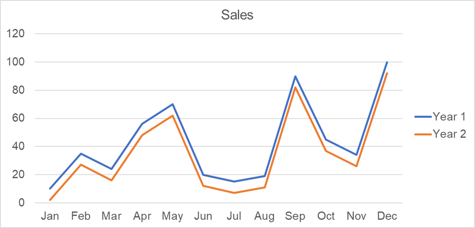
The residuals on some months are correlated - meaning, they move together. Here, this is because of seasonal trends, where shopping increases during holiday periods. Below are some ways to test for autocorrelation.
| DWH | Rule of Thumb | |
| No autocorrelation | DWH between 0 and 4 | Residual v. predicted value plot is null, or no pattern |
OLS Assumptions in Real Life
Let’s start with the first two assumptions, checked below.
| # | Assumption | Answer |
| 1 | Linear in parameters | The model is  |
| 2 | Random sample | While we’re not told about the sampling method, we can assume it is a random sample |
Next, we check assumption #4 by looking at the correlation matrix. As you could have probably guessed, our independent variables are highly correlated. This assumption is not passed.
| BP | Weight | Height | Age | |
| BP | 1 | |||
| Weight | 0.947891 | 1 | ||
| Height | 0.93656 | 0.822583 | 1 | |
| Age | 0.930753 | 0.852695 | 0.922422 | 1 |
Next, check for heteroscedasticity visually. Height exhibits a bit more variability for lower values.

The last two assumptions we can do together, as they both involve the residuals. You can run this MLR in any statistical program to get the following regression coefficients.
| Intercept | 1.270524 |
| Weight | 0.355794 |
| Height | 0.422362 |
| Age | 0.186278 |
With this information, you can calculate the Durbin-Watson by simply getting the residuals with the regression model. With a Durbin-Watson test statistic of 0.0543, which is substantially below 1, we can say the data is autocorrelated.
The table below gives the results of the DWH test.
| p-value = 1.3 | Reject null hypothesis of no endogeneity |
Based off of the multiple violations of assumptions, we should not use this model.
Summarise with AI:
Did you like this article? Rate it!


 Loading...