Linear Regression Definition
A simplified definition of linear regression boils down to measuring the degree of the linear relationship between two variables. Linear regression has a vast number of diverse, real world applications. For example, linear regression can be used to investigate the relationship between income and life satisfaction, divorce rates and crises, and much more. In order to understand some of the concepts behind linear regression, take a look at the definitions summarized in the table below.
| Concept | Definition | Formula | Example |
| Simple Linear Regression | A linear regression model that has only one independent variable |  |  |
| Pearson’s Correlation Coefficient | The measure of the strength of the relationship between two variables. |  | The correlation coefficient between exam score and study hours is 0.84, suggesting a strong relationship. |
- Simple linear regression
- Multiple linear regression
Both types of regression seek to understand the relationship between a dependent and independent variable. The only difference is that, while simple linear regression deals with only one dependent variable and one independent variable, multiple linear regression has a dependent variable with more than one independent variable. A dependent variable is defined as the variable which you are interested in studying. More specifically, this variable is the one that is effected depending on the change of value of the independent variable. This explains its name, because the value of the variable is “dependent” on the other variables. An independent variable, on the other hand, is one that is independent of other variables you are attempting to study. To understand linear regression, let's start with a step-by-step example of simple linear regression.
Linear Regression Example
In order to understand simple linear regression, we can start by breaking down the concepts used in linear regression with a step-by-step example. Note that when conducting a linear regression, you will most likely be using a program that calculates these steps for you. However, it can be helpful to do a regression by hand in order to fully grasp the ideas behind it. The table below is a data set on 8 test scores and hours spent studying for that test.
| Test Score | Hours Spent Preparing |
| 95 | 6 |
| 90 | 4 |
| 89 | 5 |
| 82 | 5 |
| 80 | 4 |
| 70 | 3 |
| 60 | 0.5 |
| 95 | 6 |
Below, you'll find the steps that you should take when calculating the linear regression line broken down by the statistics you need to calculate.
| Step | Description | Formula |
| 1 | Find the mean of x |  |
| 2 | Find the mean of y |  |
| 3 | Find the correlation of x and y | |
| 4 | Find the standard deviation of x |  |
| 5 | Find the standard deviation of y |  |
| 6 | Find the slope |  |
| 7 | Find the intercept |  |
| 8 | Find the regression model |  |
| Observation | Test Score | Hours Spent |   |   |  |  |  |
| 1 | 95 | 6 | 12.4 | 1.8 | 22.4 | 153.1 | 3.3 |
| 2 | 90 | 4 | 7.4 | -0.2 | -1.4 | 54.4 | 0.0 |
| 3 | 89 | 5 | 6.4 | 0.8 | 5.2 | 40.6 | 0.7 |
| 4 | 82 | 5 | -0.6 | 0.8 | -0.5 | 0.4 | 0.7 |
| 5 | 80 | 4 | -2.6 | -0.2 | 0.5 | 6.9 | 0.0 |
| 6 | 70 | 3 | -12.6 | -1.2 | 15.0 | 159.4 | 1.4 |
| 7 | 60 | 0.5 | -22.6 | -3.7 | 83.4 | 511.9 | 13.6 |
| 8 | 95 | 6 | 12.4 | 1.8 | 22.4 | 153.1 | 3.3 |
| Average | 82.6 | 4.2 | Total | 147.1 | 1079.9 | 23.0 |
 |  |
 |  |
 |  |
 |  |
 |  |
 |  |
Residuals
Residuals can be used as an important indicator of whether or not our regression model is a good fit for our data. First, we can start by plotting our regression model from the previous example. 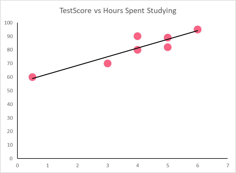
| Concept | Definition | Notation | Description |
| Residual | The difference between what the regression line predicts and what is plotted by the scatter plot |  | Residual = observed y - predicted y |
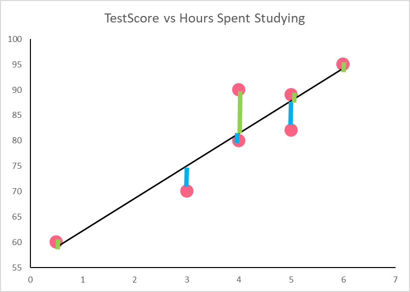

’s are found by simply plugging in the same hours into the regression model
| yi | yhat | Residual | Interpretation |
| 95 | 94.2 | 0.8 | Positive residuals indicate it is over predicted by the regression model |
| 90 | 81.4 | 8.6 | Overestimated |
| 89 | 87.8 | 1.2 | Overestimated |
| 82 | 87.8 | -5.8 | Negative residuals indicate it is r predicted by the regression model |
| 80 | 81.4 | -1.4 | Underestimated |
| 70 | 75.0 | -5.0 | Underestimated |
| 60 | 59.0 | 1.0 | Overestimated |
| 95 | 94.2 | 0.8 | Overestimated |
Summarise with AI:
Did you like this article? Rate it!


 Loading...