Multiple linear regression is the extension of simple linear regression and is equally as common in statistics. To understand how multiple linear regression analysis works, try to solve the following problem by reviewing what you already know and reading through this guide. This guide is meant for those unsure how to approach the problem or for those encountering this concept for the first time.






Problem 5
You’re curious about which factors play into the salary people earn. In order to find out you’d like to conduct a multiple linear regression analysis on data that has the salary, education level in years, and work experience for 10 individuals. Conduct a multiple regression analysis by finding the regression model on the following data set.
| Education | Experience | Salary |
| 11 | 10 | 30000 |
| 11 | 6 | 27000 |
| 12 | 10 | 20000 |
| 12 | 5 | 25000 |
| 13 | 5 | 29000 |
| 14 | 6 | 35000 |
| 14 | 5 | 38000 |
| 16 | 8 | 40000 |
| 16 | 7 | 45000 |
| 16 | 2 | 28000 |
| 18 | 6 | 30000 |
| 18 | 2 | 55000 |
| 22 | 5 | 65000 |
| 23 | 2 | 25000 |
| 24 | 1 | 75000 |
What is MLR?
Multiple linear regression is the extension of simple linear regression. Meaning, the basic concepts behind multiple linear regression, or MLR, are the same. The main difference, however, is that multiple linear regression has one response variable with two or more explanatory variables.
The motivation behind MLR is that in many cases, the predictions from regression models get better with more explanatory variables. Intuitively, this makes sense as the majority of the phenomena around us - the demand for goods, the growth of plants, etc. - typically have more than just one variable related to them. Mathematically, this also makes sense: the more variables you add to the model, the higher the explained variance, or R squared value, of the model.
However, introducing more variables means you should practice extra precaution during your analysis. Having a high r-squared value doesn’t always mean you’ve found the best regression model. Often, too high of an r-squared value can signal towards underlying problems with your model. Take a look at some of the common problems you can encounter when building your MLR model.
| Concept | Definition | Resulting Problems |
| Overfitting | Adding too many predictors | The model is too closely related, or “fit”, to the sample data set to the point that it introduces a lot of variability |
| Underfitting | Adding too few predictors | The model does not “fit” the data well enough because it is not complex enough to the point that it introduces bias |
| Multicollinearity | Pairs of explanatory variables are too highly correlated | Reduces the reliability of the model because it affects the variance |
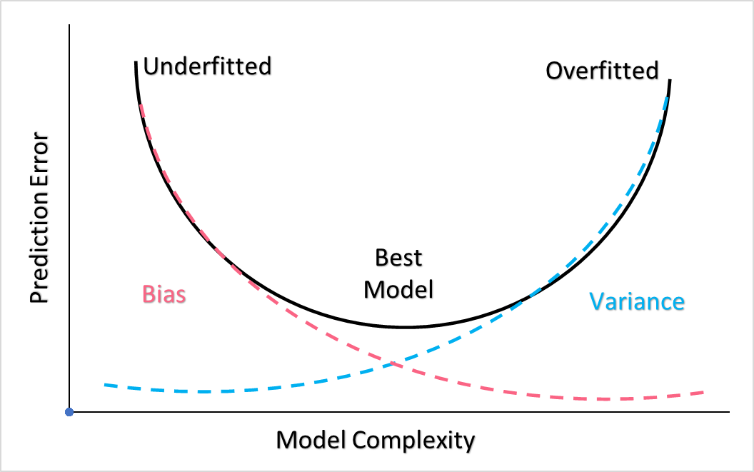
The first two concepts are often referred to as the bias-variance trade-off. The more complex your model, the higher the risk of overfitting the data and therefore having higher variance. The less complex the model, the higher the risk of underfitting the data and therefore the having higher bias. The best models find the sweet spot between the overfitted and underfitted model, which can be visualized in the graph below.
MLR Explained
In order to explain multiple linear regression, let’s start with the multiple regression model.
[
y = beta_{0} + beta_{1}x_{1} + beta_{2}x_{2} + beta_{3}x_{3} + … + beta_{n}x_{n} + u_{i}
]
As you may notice, this is simply an extension of the SLR model, which can be written in any of the following ways.
 |
 |
 |
 |
In order to understand this equation, let's break it down by first looking at the linear parameters.

Find a summary of these linear parameters below
| Linear Parameter | Description |
 | The intercept |
 | The regression coefficient of the first independent variable |
 | The regression coefficient of the second independent variable |
 | The regression coefficient of the  th independent variable th independent variable |
Next, take a look at the error term.

Recall that this error term is based off of the real population parameters. In the MLR equation, this error term is actually assumed to be zero. Because we do not know the true population parameters, we arrive at the estimated multiple regression equation.
[
hat{y} = b_{0} + b_{1}x_{1} + b_{2}x_{2} + b_{3}x_{3} … + b_{n}x_{n}
]
Take a look at the table below to understand what this estimated MLR equation means.
| Estimated Parameter | Description |
 | The estimates of the population parameters  |
 | The estimate of the parameter  |
Remember that the population parameters are measured from the actual population, whereas the estimates of these parameters are based off of a sample from the population and they are called statistics.
MLR Estimators
To calculate the estimators, let’s start with the easiest first, which is the intercept. The equation for the intercept is simply a rearranged version of the MLR equation. To illustrate this, take an MLR equation with only two independent variables.
[
y = b_{0} + b_{1}x_{1 + b_{2}x_{2}}
]
Solving for  , we get:
[
b_{0} = bar{y} - b_{1}bar{x_{1}} - b_{2}x_{2}}
]
The formulas for the  and
and  estimators are a bit more complicated. Take a look at the table below to see the formulas you’ll need to calculate these estimators.
| Element | Formula |
|  |
|  |
 |  |
 |  |
Two Variable MLR Step by Step
| Observation | Salary | Education | Experience |  |  |  |  |  |
| 1 | 30000 | 11 | 10 | 121 | 100 | 330000 | 300000 | 110 |
| 2 | 27000 | 11 | 6 | 121 | 36 | 297000 | 162000 | 66 |
| 3 | 20000 | 12 | 10 | 144 | 100 | 240000 | 200000 | 120 |
| 4 | 25000 | 12 | 5 | 144 | 25 | 300000 | 125000 | 60 |
| 5 | 29000 | 13 | 5 | 169 | 25 | 377000 | 145000 | 65 |
| 6 | 35000 | 14 | 6 | 196 | 36 | 490000 | 210000 | 84 |
| 7 | 38000 | 14 | 5 | 196 | 25 | 532000 | 190000 | 70 |
| 8 | 40000 | 16 | 8 | 256 | 64 | 640000 | 320000 | 128 |
| 9 | 45000 | 16 | 7 | 256 | 49 | 720000 | 315000 | 112 |
| 10 | 28000 | 16 | 2 | 256 | 4 | 448000 | 56000 | 32 |
| 11 | 30000 | 18 | 6 | 324 | 36 | 540000 | 180000 | 108 |
| 12 | 55000 | 18 | 2 | 324 | 4 | 990000 | 110000 | 36 |
| 13 | 65000 | 22 | 5 | 484 | 25 | 1430000 | 325000 | 110 |
| 14 | 25000 | 23 | 2 | 529 | 4 | 575000 | 50000 | 46 |
| 15 | 75000 | 24 | 1 | 576 | 1 | 1800000 | 75000 | 24 |
| Total | 567000 | 240 | 80 | 4096 | 534 | 9709000 | 2763000 | 1171 |
| Mean | 37800 | 16 | 5 |
Next, we go ahead and plug them in.
[
sum x_{1}^2 = 4096 - frac{(240)^2}{15} = 256
]
[
sum x_{2}^2 = 534 - frac{(80)^2}{15} = 107
]
[
sum x_{1}y = 9709000 - frac{567000*240}{15} = 637000
]
[
sum x_{2}y = 2763000 - frac{567000*80}{15} = -261000
]
[
sum x_{1}x_{2} = 1171 - frac{240*80}{15} = -109
]
[
b_{1} = frac{(107*637000) - (-109* -261000)}{(256*107) - (-109)^2} = 2560
]
[
b_{2} = frac{(256*-261000) - (-109*637000)}{(256*107) - (-109)^2} = 168
]
[
b_{0} = 37800 - (2560*16) - (168*5) = -4051
]
Putting these numbers all together, we get a multiple regression model of:
[
y = -4051 + 2560x_{1} + 168x_{2}
]
Summarise with AI:
Did you like this article? Rate it!


 Loading...