Standard deviation is one of the most important measures in statistics, yet it is often misunderstood. In this article, we explain what standard deviation is, how to calculate it for both ungrouped and grouped data, and how to interpret the result in context. We also walk through the relationship between standard deviation and variance, cover key characteristics of the measure, and provide fully worked examples throughout.


What is Standard Deviation?
The standard deviation (often abbreviated as SD) is a measure of variability in descriptive statistics. It tells us how much the values in a data set are spread out from the mean. Two key rules of thumb apply:
- The lower the standard deviation, the closer the values are to the mean and the less variability there is.
- The higher the standard deviation, the farther the values are spread from the mean and the more variability there is.
In practical terms, a small standard deviation means the data points cluster tightly around the average, while a large standard deviation means they are widely scattered.
Population vs Sample Standard Deviation
The formula for standard deviation depends on whether you are working with an entire population or a sample drawn from a population. Another useful shortcut: the variance is simply the square of the standard deviation, so if you already know the variance, you can find the SD by taking the square root.
The table below summarises the notation and formulas for each.
| Measure | Population | Sample |
|---|---|---|
| Standard Deviation Notation | σ | s |
| Standard Deviation Formula | σ = √[ Σ(xᵢ − μ)² / N ] | s = √[ Σ(xᵢ − x̄)² / (n−1) ] |
| Variance Notation | σ² | s² |
| Variance Formula | σ² = Σ(xᵢ − μ)² / N | s² = Σ(xᵢ − x̄)² / (n−1) |
Notice that for a sample, we divide by  rather than
  . This is called Bessel's correction and it ensures the sample standard deviation is an unbiased estimator of the population standard deviation. In the formulas above,
  is the population mean,
  is the sample mean,
  is the population size, and is the sample size.
How to Calculate the Standard Deviation for Grouped Data
Often, data is presented in grouped form rather than as individual values. For example, test scores might be grouped into categories such as 10–20, 20–30, and so on. When the data is grouped, we do not know the exact value of each observation, so we use the midpoint of each class interval as a representative value.
The formula for the sample grouped standard deviation is:

where  is the midpoint of each group,
  is the frequency of each group, is the grouped mean, and is the total number of observations.
Step-by-Step Method
| Step | Description | Formula |
|---|---|---|
| 1 | Find the midpoint of each group | xₘ = (lower bound + upper bound) / 2 |
| 2 | Multiply each midpoint by its frequency | xₘ × fᵢ |
| 3 | Sum the products and divide by n to get the grouped mean | x̄ = Σ(xₘ × fᵢ) / n |
| 4 | Subtract the grouped mean from each midpoint | xₘ − x̄ |
| 5 | Square each deviation | (xₘ − x̄)² |
| 6 | Multiply each squared deviation by its frequency | fᵢ × (xₘ − x̄)² |
| 7 | Sum all the weighted squared deviations | Σ fᵢ × (xₘ − x̄)² |
| 8 | Divide by (n − 1) | Σ fᵢ(xₘ − x̄)² / (n − 1) |
| 9 | Take the square root | √[ Σ fᵢ(xₘ − x̄)² / (n − 1) ] |
Worked Example: Test Scores
A classroom's test scores are grouped as follows:
| Test Score Categories | Frequency |
|---|---|
| 10 – 20 | 1 |
| 20 – 30 | 8 |
| 30 – 40 | 5 |
| 40 – 50 | 9 |
| 50 – 60 | 8 |
| 60 – 70 | 10 |
| 70 – 80 | 75 |
| Total | 116 |
Following the step-by-step method, we build the calculation table:
| Test Score Categories | Frequency (f) | Midpoint (xₘ) | xₘ × f | xₘ − x̄ | (xₘ − x̄)² | f × (xₘ − x̄)² |
|---|---|---|---|---|---|---|
| 10 – 20 | 1 | 15 | 15 | −49.7 | 2,474.2 | 2,474.2 |
| 20 – 30 | 8 | 25 | 200 | −39.7 | 1,579.4 | 12,635.0 |
| 30 – 40 | 5 | 35 | 175 | −29.7 | 884.5 | 4,422.7 |
| 40 – 50 | 9 | 45 | 405 | −19.7 | 389.7 | 3,507.5 |
| 50 – 60 | 8 | 55 | 440 | −9.7 | 94.9 | 759.2 |
| 60 – 70 | 10 | 65 | 650 | 0.3 | 0.1 | 0.7 |
| 70 – 80 | 75 | 75 | 5,625 | 10.3 | 105.2 | 7,892.9 |
| Total | 116 | 7,510 | 31,692.2 |
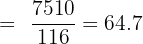
First, calculate the grouped mean:
Then calculate the grouped standard deviation:
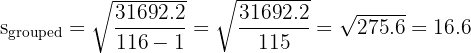
The grouped standard deviation is approximately 16.6.
Characteristics of Standard Deviation
The standard deviation has several properties that always hold true:
- The standard deviation is always zero or positive. It can never be negative because it is calculated from squared values.
- The standard deviation is zero if and only if every value in the data set is equal to the mean (i.e. there is no variability at all).
- The standard deviation is sensitive to outliers. A single extreme value can significantly increase the SD.
Interpreting the Standard Deviation
A higher standard deviation means greater variability, but that is not always a "bad" thing. Interpreting the SD depends entirely on the context of the data and the question you are trying to answer.
Consider two restaurants that ask customers to rate each dish on a scale from 0 to 100.
| Dish | Restaurant A (score) | Restaurant B (score) |
|---|---|---|
| Pasta | 20 | 60 |
| Salad | 10 | 90 |
| Rice | 30 | 70 |
| Burger | 25 | 80 |
| Mean | 21.25 | 75.0 |
| SD (population) | 7.4 | 11.2 |
Restaurant A has a lower standard deviation (7.4) than Restaurant B (11.2), meaning its ratings are more consistent. However, the ratings are consistently low — an average of just 21.25 out of 100. Restaurant B has more variability in its scores, but its mean rating is 75.0, which is much higher. In this case, the higher variability comes with a much better average outcome.
The lesson is clear: always consider the standard deviation alongside other statistics such as the mean, and always interpret it in the context of the problem.
Problem 1: Grouped Standard Deviation
You are studying how many hours per week students spend on social media. A study of 65 students produced the following grouped data. Find and interpret the grouped standard deviation, rounding to the nearest tenth.
| Number of Hours | Number of Students |
|---|---|
| 0 – 2 | 5 |
| 2 – 4 | 13 |
| 4 – 6 | 24 |
| 6 – 8 | 17 |
| 8 – 10 | 6 |
Solution to Problem 1
The number of students in each category is the frequency, and the total number of students is our sample size,  .
.
| Hours | Students (f) | Midpoint (xₘ) | xₘ × f | xₘ − x̄ | (xₘ − x̄)² | f × (xₘ − x̄)² |
|---|---|---|---|---|---|---|
| 0 – 2 | 5 | 1 | 5 | −4.2 | 17.5 | 87.6 |
| 2 – 4 | 13 | 3 | 39 | −2.2 | 4.8 | 62.0 |
| 4 – 6 | 24 | 5 | 120 | −0.2 | 0.0 | 0.8 |
| 6 – 8 | 17 | 7 | 119 | 1.8 | 3.3 | 56.0 |
| 8 – 10 | 6 | 9 | 54 | 3.8 | 14.6 | 87.3 |
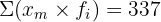
| Total | 65 | 337 | 293.8 |
Step by step:
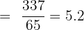
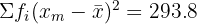
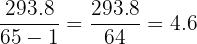
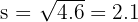
The grouped standard deviation is approximately 2.1 hours.
Interpretation: On average, students' weekly social media usage deviates from the mean (5.2 hours) by about 2.1 hours. This suggests that most students spend between roughly 3 and 7 hours per week on social media, which is a moderate level of variability.
Additional Problems
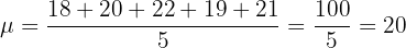
The ages of five members of a quiz team are 18, 20, 22, 19, and 21. Calculate the population standard deviation.
First, find the mean:
Calculate each squared deviation:

Sum the squared deviations:

Divide by  :
:
Take the square root:
The population standard deviation is approximately 1.41 years.
A student measures the time (in seconds) it takes to run 100 metres on six occasions: 12.4, 12.8, 12.1, 13.0, 12.6, 12.5. Calculate the sample standard deviation.
Find the sample mean:

Calculate each squared deviation (rounding to 3 decimal places):
Sum:

Divide by  :
:
Take the square root:
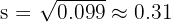
The sample standard deviation is approximately 0.31 seconds. This is a small value relative to the mean, indicating that the student's sprint times are quite consistent.
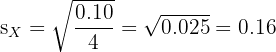
Two factories produce bolts. A sample of 5 bolts from each factory is measured for length (in mm). Factory X: 50.1, 49.9, 50.0, 50.2, 49.8. Factory Y: 51.0, 48.5, 50.5, 49.0, 51.0. Which factory produces more consistent bolts?
Factory X:


Factory Y:


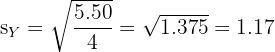
Both factories produce bolts with the same mean length (50.0 mm), but Factory X has a standard deviation of 0.16 mm compared to Factory Y's 1.17 mm. Factory X produces much more consistent bolts.
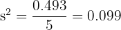
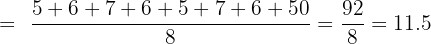
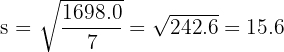
A data set contains the values 5, 6, 7, 6, 5, 7, 6, 50. Calculate the sample standard deviation with and without the outlier (50).
With the outlier (n = 8):

Without the outlier (n = 7):
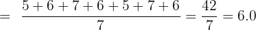

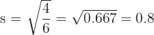
The standard deviation drops from 15.6 to 0.8 when the outlier is removed. This demonstrates how dramatically a single extreme value can inflate the standard deviation and why it is important to identify outliers before interpreting your results.
The annual salaries (in thousands of pounds) of employees at a small company are grouped below. Find the grouped sample standard deviation.
| Salary Range (£000s) | Number of Employees |
|---|---|
| 20 – 30 | 4 |
| 30 – 40 | 10 |
| 40 – 50 | 15 |
| 50 – 60 | 8 |
| 60 – 70 | 3 |

| Salary Range | f | xₘ | xₘ × f | xₘ − x̄ | (xₘ − x̄)² | f × (xₘ − x̄)² |
|---|---|---|---|---|---|---|
| 20 – 30 | 4 | 25 | 100 | −19.0 | 361.0 | 1,444.0 |
| 30 – 40 | 10 | 35 | 350 | −9.0 | 81.0 | 810.0 |
| 40 – 50 | 15 | 45 | 675 | 1.0 | 1.0 | 15.0 |
| 50 – 60 | 8 | 55 | 440 | 11.0 | 121.0 | 968.0 |
| 60 – 70 | 3 | 65 | 195 | 21.0 | 441.0 | 1,323.0 |
| Total | 40 | 1,760 | 4,560.0 |
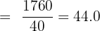
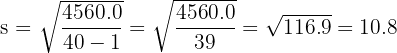
The grouped standard deviation is approximately £10,800. This tells us that employee salaries typically deviate from the mean of £44,000 by about £10,800.
Summarise with AI:
Did you like this article? Rate it!


Can you help me answer my activities