Frequency
Frequency is defined as the amount of times a value occurs. To illustrate this, let’s start by looking at a table, which shows the number of times someone bought a given phone model.
| Model | Count |
| A1 | IIIII IIIII |
| S4 | IIIII |
| D5 | IIIII IIIII IIIII |
| F6 | IIIII IIIII IIIII IIIII IIIII |
| J9 | IIIII II |
In order to calculate the frequency, you simply need to add all of the times the model has been bought, which can be seen in the ‘Count’ column. See the final frequencies below.
| Model | Frequency |
| A1 | 10 |
| S4 | 5 |
| D5 | 15 |
| F6 | 25 |
| J9 | 7 |
Frequencies are helpful because they can help us understand the distribution of the data.
Frequency Distribution
Continuing from the previous example, a frequency distribution is a function or a graph that helps us see the distribution of a variable. A distribution is the way something is spread or shared. Take a look at the graph below, which shows the distribution of the phones that have been bought. 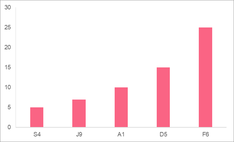
| Height | Frequency |
| 150 | 2 |
| 155 | 3 |
| 160 | 9 |
| 165 | 12 |
| 170 | 20 |
| 175 | 25 |
| 180 | 25 |
| 185 | 10 |
| 190 | 18 |
| 195 | 20 |
| 200 | 5 |
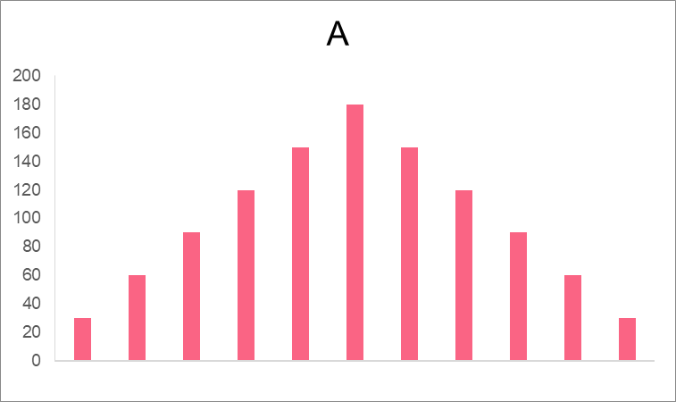
As you can see, displaying the frequency of more than a couple of categories or values. This is where a frequency distribution can come in handy. The image below shows a frequency distribution of the example heights. 
| Graph | Type | Description |
| A | Unimodal | Has one peak, where values are cantered |
| B | Bimodal | Has two peaks, which illustrate the two centres in the data |
| C | Multimodal | Has multimodes, which illustrate multiple points around which values in the data centre |


Probability
The probability of an event is the likelihood of that event happening. This probability, however, depends on what type of event it is. The table below summarizes the formulas for the probability of different types of events.
| Notation | Formula | |
| 1 event | P(A) |  |
| 2 independent events |  | P(A) * P(B) |
| 2 dependent events | | P(A) * P(B|A) |
| 2 mutually exclusive events |  | P(A) + P(B) |
| 2 not mutually exclusive events | | P(A) + P(B) - P(A B) |
Probability Distribution
A probability distribution is a formula or visualization that tells us the probability of an event occurring. The image below shows the probability distribution of landing on heads when flipping a coin 5 times. 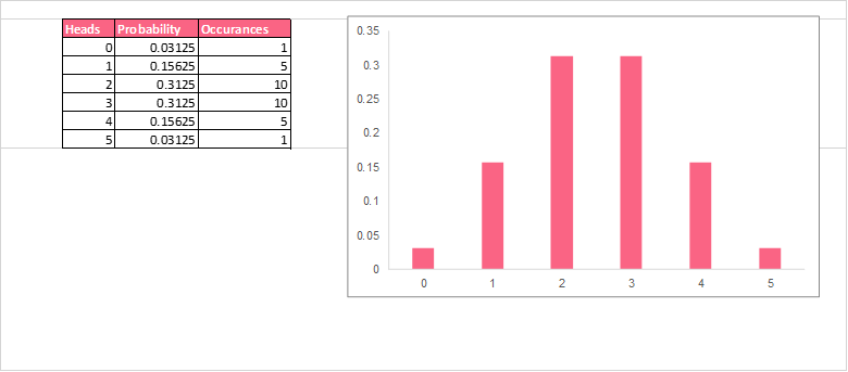
| Heads | Probability | Probability |
| 0 |  | 0.06 |
| 1 |  | 0.25 |
| 2 |  | 0.38 |
| 3 |  | 0.25 |
| 4 |  | 0.06 |
Types of Distributions
There are many types of probability distributions. The three most common ones can be seen in the images below.


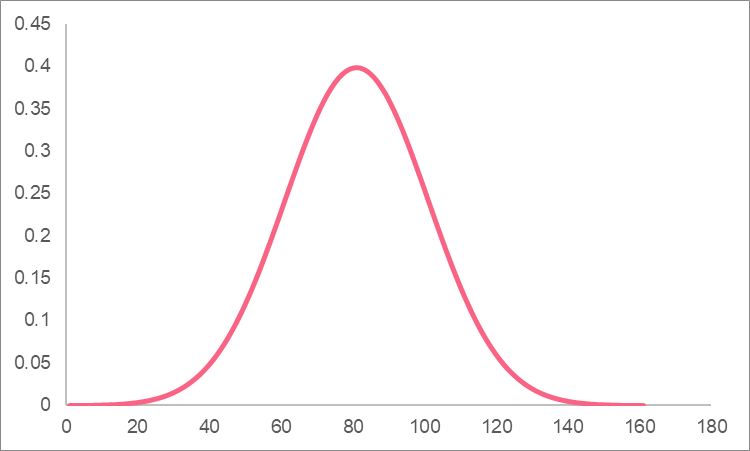
As you can see, these distributions are similar to the one in the previous example. However, finding the probability of a single value can be performed using formulas instead of mechanically. These formulas are the following.
| Mean | Other Parameters | Probability Equation | |
| Standard normal | Mean = | SD = , x = test value | z = , probability found on z-table |
| Binomial | n = # of trials | p = probability of success in each trial, q = 1-p, x = test value |  |
| Poisson | Mean = | x = test value | P = |
Standard Normal Distributions
The most common type of distribution that you will encounter in statistics classes is the standard normal distribution. This distribution standardizes the values for a variable that has a normal distribution. It does this by taking the plain numbers, known as “raw scores,” and plugging them into the following formulas.
| Population Parameters | Sample Statistics | |
| Formula | |  |
Z-score
Another name for the standardized value found from the standardisation formula above is a z-score. Z-scores are vital for finding the probability of a value in a standard normal distribution because they let us know how far away any given value is from the mean. Take a look at the standard normal distribution below. 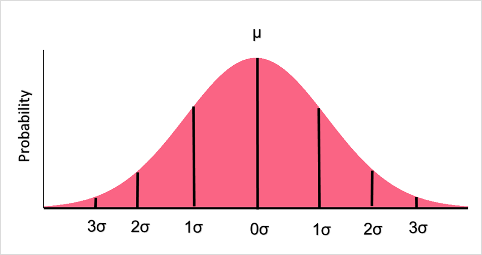
| Mean | Standard Deviation | Value 1 SD Above the Mean | Z-score |
| 30 | 4 | 30 + 4 |  = 1 |
| 30 | 10 | 30 + 10 |  = 1 |
| 30 | 100 | 30 + 100 |  = 1 |
Z-table
Calculating the z-score is only one half of finding the probability. As you can see in the image above, each z-score corresponds to a probability, which is written down in a z-table. A z-table is either right or left tailed, which depends on whether or not you are finding the probability above, below or of an interval of any values. 
| When | Graph | |
| Right-tail | Of or above a value | C,D |
| Left-tail | Of or below a value | A,B |
Standard Normal Example
You are interested in knowing the probability of getting 1000 points for an exam that has a mean of 850 and a standard deviation of 100. First, you find the z-score. \[ z-score = \frac{1000-850}{100} = 1.50 \] Next, we look up this value in a left tail z-table. This is because we are scoring up to 1000 points, not above 1000. 
Summarise with AI:
Did you like this article? Rate it!

 Loading...