In fields like economics, engineering, and data science, efficiency is everything. Businesses want to maximise their profits while minimising production costs. Aerospace engineers design wing profiles to maximise lift while minimising aerodynamic drag. In mathematics, these real-world objectives are modelled as functions, and the peaks and troughs of these functions are known as extrema (maxima and minima).
While sketching a curve allows us to locate these points visually, drawing highly complex functions accurately is time-consuming. Calculus provides a precise, analytical shortcut. By using differentiation, we can systematically pinpoint the exact coordinates where a system reaches its peak performance or its absolute lowest threshold.


Core Theory: Stationary Points
A stationary point (or turning point) occurs on a curve where the gradient is exactly zero. If you were to draw a tangent line to the curve at these specific locations, the line would be completely horizontal.
In calculus notation, for a function , stationary points are located by solving the first derivative equation:
The Three Profiles of Stationary Points
- Local Maximum: The highest point in its immediate neighbourhood. As the curve passes through a maximum, the gradient changes from positive (climbing), to zero (at the peak), to negative (falling).
- Local Minimum: The lowest point in its immediate neighbourhood. As the curve passes through a minimum, the gradient changes from negative (falling), to zero (at the trough), to positive (climbing).
- Stationary Point of Inflexion: A point where the curve flattens out momentarily, , but then continues in its original direction. The gradient does not change sign; it goes from positive to zero to positive, or from negative to zero to negative.
Deducing the Nature: The Two Derivative Tests
Finding the x-coordinate where tells you where a turning point is, but it does not tell you what type of point it is. To determine its nature under exam conditions, you have two primary methods.
Method A: The Second Derivative Test
This is the fastest and most common method used at A-Level. The second derivative, written as:
or , measures the rate of change of the gradient (the concavity of the curve).
- If at the stationary point, the gradient is decreasing. The curve is concave down, meaning the point is a local maximum.
- If at the stationary point, the gradient is increasing. The curve is concave up, meaning the point is a local minimum.
Crucial Exam Warning: If [/latex], the test is completely inconclusive. The point could be a maximum, a minimum, or a point of inflexion (for example, and both yield a second derivative of zero at x = 0, but have entirely different natures). In this scenario, you must fall back on Method B.
Method B: The First Derivative Test (Gradient Sign Table)
This method involves analyzing the sign of the first derivative at points slightly to the left and slightly to the right of your stationary value.
| Point Location | Left of Stationary Point | At Stationary Point | Right of Stationary Point | Resulting Shape |
|---|---|---|---|---|
| Maximum Profile | Positive (+) | Zero (0) | Negative (-) | Inverted U-Shape (Peak) |
| Minimum Profile | Negative (-) | Zero (0) | Positive (+) | U-Shape (Trough) |
| Inflexion (Rising) | Positive (+) | Zero (0) | Positive (+) | S-Shape Flat Link |
Systematic Execution Matrix
To solve any standard calculus extrema problem, use this step-by-step operational roadmap:
| Step | Operational Task | Mathematical Action |
|---|---|---|
| 1 | Differentiate once | Find the first derivative expression: f'(x) |
| 2 | Find Critical Roots | Set f'(x) = 0 and solve the resulting equation for x |
| 3 | Differentiate twice | Find the second derivative expression: f''(x) |
| 4 | Test and Classify | Substitute your x-roots into f''(x) to verify if the output is positive or negative |
| 5 | Find Coordinate Pairs | Substitute the valid x-roots back into the *original* y = f(x) function to find the matching y-values |
Exam-Style Optimisation Problems
Problem 1: Pure Algebraic Extrema
Find the coordinates of the stationary points on the curve given by:
and determine their nature using the second derivative test.
Find the first derivative:
Set the expression equal to zero and solve for the roots:
This gives two critical stationary coordinates: x = 2 and x = -1.
Find the second derivative:
Test the nature of each root:
- For x = -1:
Since -18 < 0, this point is a local maximum.
- For x = 2:
Since 18 > 0, this point is a local minimum.
Calculate the matching y-coordinates from the original equation:
Conclusion: The local maximum coordinate is (-1, 12). The local minimum coordinate is (2, -15).
Problem 2: Applied Geometric Optimisation
A manufacturing firm needs to construct an open-topped storage box with a square base of length x cm and a vertical height of h cm. The total surface area of the sheet metal used to construct the box is fixed at exactly .
- Show that the volume V of the box is given by the formula:
- Use calculus to find the maximum possible volume of the box, justifying that your answer is a maximum.
Part 1: Setting up the constraint formulas
- The volume of the box is:
- The surface area consists of 1 square base and 4 identical rectangular sides:
Isolate h from the surface area equation to remove it from the volume model:
Substitute this expression for h back into the volume formula:
Part 2: Optimising the volume expression
Differentiate V with respect to x:
Set to find the maximum volume configuration:
(Note: We disregard the negative root x = -10 because a physical length measurement must be positive).
Verify the nature of this root using the second derivative test:
At
Since -15 < 0, the volume is definitively maximised when x = 10.
Calculate the final maximum volume value:
Examiner Tips & Common Pitfalls
Examiner Tip: A highly frequent source of lost marks in A-Level optimisation contexts is failing to complete Step 5. Students often calculate the correct optimal value for x, prove it is a maximum, and immediately move on to the next question without actually substituting x back into the function to find the maximum value of y (or Volume/Profit) requested by the wording of the prompt.
Additionally, always pay attention to the domain boundaries of a function. If an optimisation function yields a critical value that sits completely outside the physical domain of the scenario (e.g., a negative radius, or an asymptote where the function is completely undefined), that candidate root must be formally excluded from your final analysis.
Practice Questions & Solutions
Find the stationary points of the function:

and classify their nature.
First, find the derivative expression:

Set the derivative equal to zero to find the critical roots:

Find the second derivative expression to test the nature of the turning points:
f''(x) = 6x
Evaluate at x = 1:
f''(1) = 6(1) = 6 > 0 Local Minimum.
Evaluate at x = -1:
 Local Maximum.
Find the corresponding outputs for the original function:


Therefore, the local maximum is at (-1, 4) and the local minimum is at (1, 0).
A firm's weekly total revenue model is modeled by: 
where x is the number of units manufactured per week. Find the production volume x that yields the maximum possible revenue.
Differentiate the revenue expression with respect to the production volume parameter:
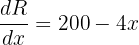
Set this expression equal to zero to optimize for peak revenue generation:

Verify that this point represents a maximum using the second derivative operation:

Since -4 <0 globally across all values, the production volume of 50 units guarantees a maximum revenue condition.< p>
Find the absolute minimum value of the rational function:
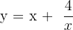
restricted to the positive domain boundary x > 0.
Rewrite the fraction using index notation to prepare for differentiation:

Differentiate the function terms:
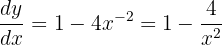
Set the expression equal to zero to locate the stationary coordinates:

Since the problem restricts the domain exclusively to positive values (x > 0), the root x = -2 is discarded. Find the second derivative to verify its nature:
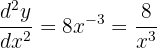
Substitute x = 2:
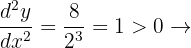
Local Minimum. Calculate the final minimum coordinate value:
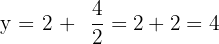
The absolute minimum value of the function on this domain is 4.
Determine the coordinate position of the stationary point on the exponential curve:

located within the positive interval x > 0.
Use the product rule to differentiate the function expression, let:

and let:


Set the derivative expression equal to zero to identify the roots:

Since the exponential multiplier:

can never equal zero, we solve the remaining polynomial factor:

Since the question asks for the stationary point situated where x > 0, we select x = 2. Find the matching y-value by substituting x = 2 into the original expression:

The target stationary coordinate pair is located at:
 .
.
Explain why the second derivative test fails to determine the nature of the stationary point at the origin for the function:

and show how the first derivative test resolves its nature.
Differentiating the function twice gives:

and
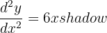 .
.
At the origin (x = 0), the second derivative evaluates to zero, which makes the test completely inconclusive. To apply the first derivative test, evaluate the gradient slightly on either side of the stationary point at x = 0:
 (Positive gradient).
At the turning point:
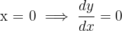 (Zero gradient).
 (Positive gradient).
Since the gradient does not change sign as it passes through the origin (remaining positive on both sides), the point is classified as a stationary point of inflexion.
Summarise with AI:
Did you like this article? Rate it!


 Loading...
I get it somehow, there are others who are unfamiliar and I have a hard time with it but it’s okay that I get it.
Thanks for sharing your thoughts! It’s completely normal to find some parts unfamiliar or more difficult than others. The important thing is that you’re making progress and understanding more as you practise. Keep going! 😊
At least I understood some of it, but there are others that I’m confused about and have a hard time understanding, but I get it.
Thanks for sharing! It’s great that you’ve understood some of it already. Don’t worry if a few parts are still confusing — keep practising and take your time with the trickier sections. You’ll get there! 😊
The lesson was a little difficult for me, especially the word problems, but the examples helped me understand it better.
Thanks for your feedback! Word problems can definitely be tricky, so we’re glad the examples helped make the lesson clearer. Keep practising — it gets easier with time! 😊
Thankyouuu po