A linear function is a first-degree polynomial function describing a relationship between an independent input variable (x) and a dependent output variable (y or f(x)) where the rate of change remains strictly constant. When plotted on a Cartesian coordinate grid, every linear function produces a continuous straight line that extends infinitely in both directions.
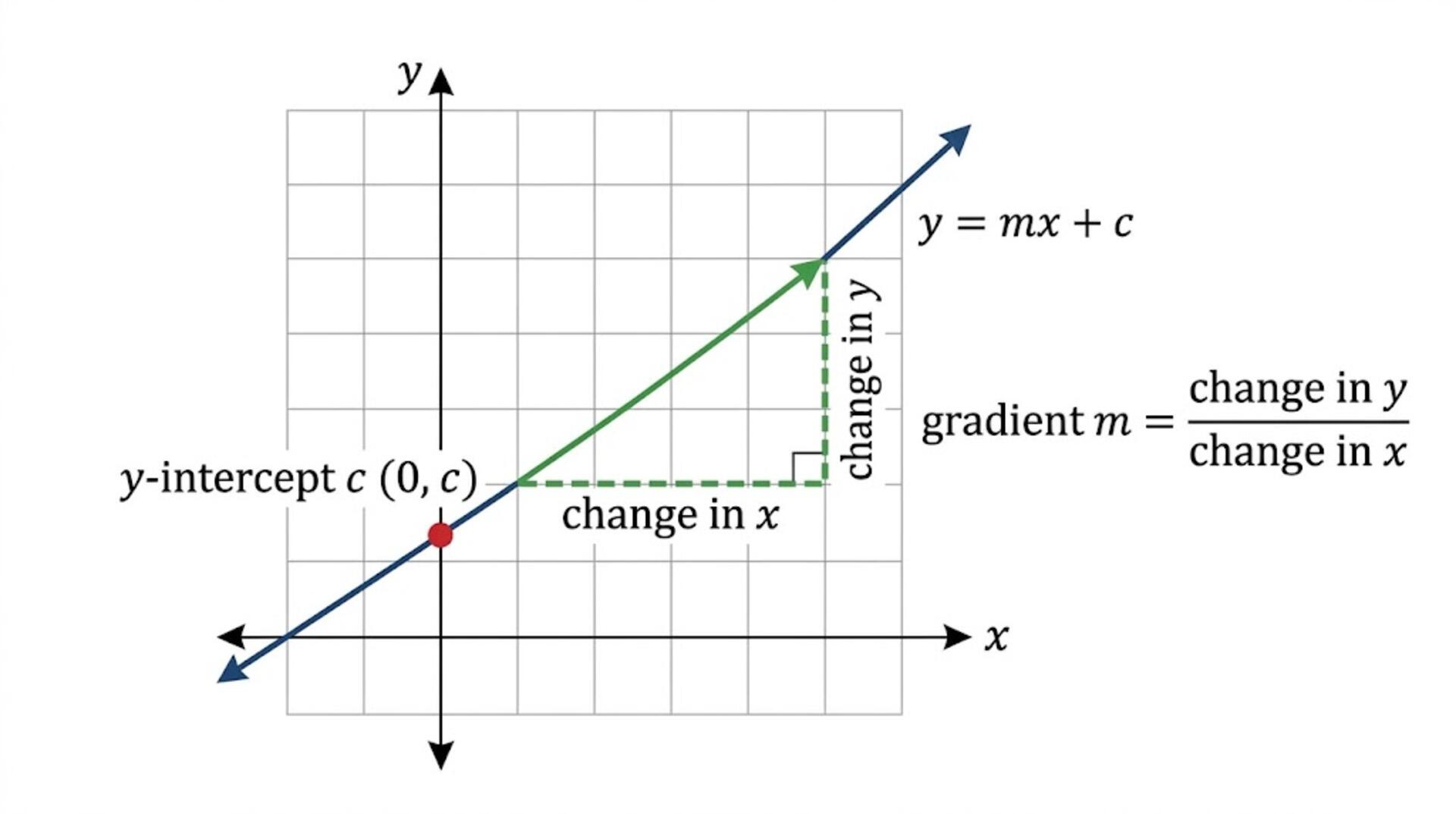
The standard algebraic equation of a linear function is:
Where:
- x is the input variable (domain).
- y or f(x) is the output variable (range).
- m is the gradient (slope), defining the steepness and direction of the line.
- c is the y-intercept, defining the point (0, c) where the line intersects the vertical y-axis.
Why Linear Functions Matter
- Real-World Applications: Linear functions model systems with constant rates of change—such as fixed-plus-variable billing systems (e.g., electricity tariffs, taxi fares), distance-time relationships under uniform velocity, and temperature conversions between Celsius and Fahrenheit.
- Academic Relevance: Linear equations are the cornerstone of coordinate geometry, vector algebra, and introductory calculus. In differential calculus, non-linear curves are analyzed locally by approximating them as linear tangent lines ().


Core Theory
The Anatomy of a Linear Equation
The most direct way to recognize a linear function is by examining the power of the variable:
- In a linear function, the variable x has an exponent of exactly 1 ().
- There are no products of variables (e.g., xy), no variables in denominators (e.g., ), and no roots or transcendental functions (e.g., , , ).
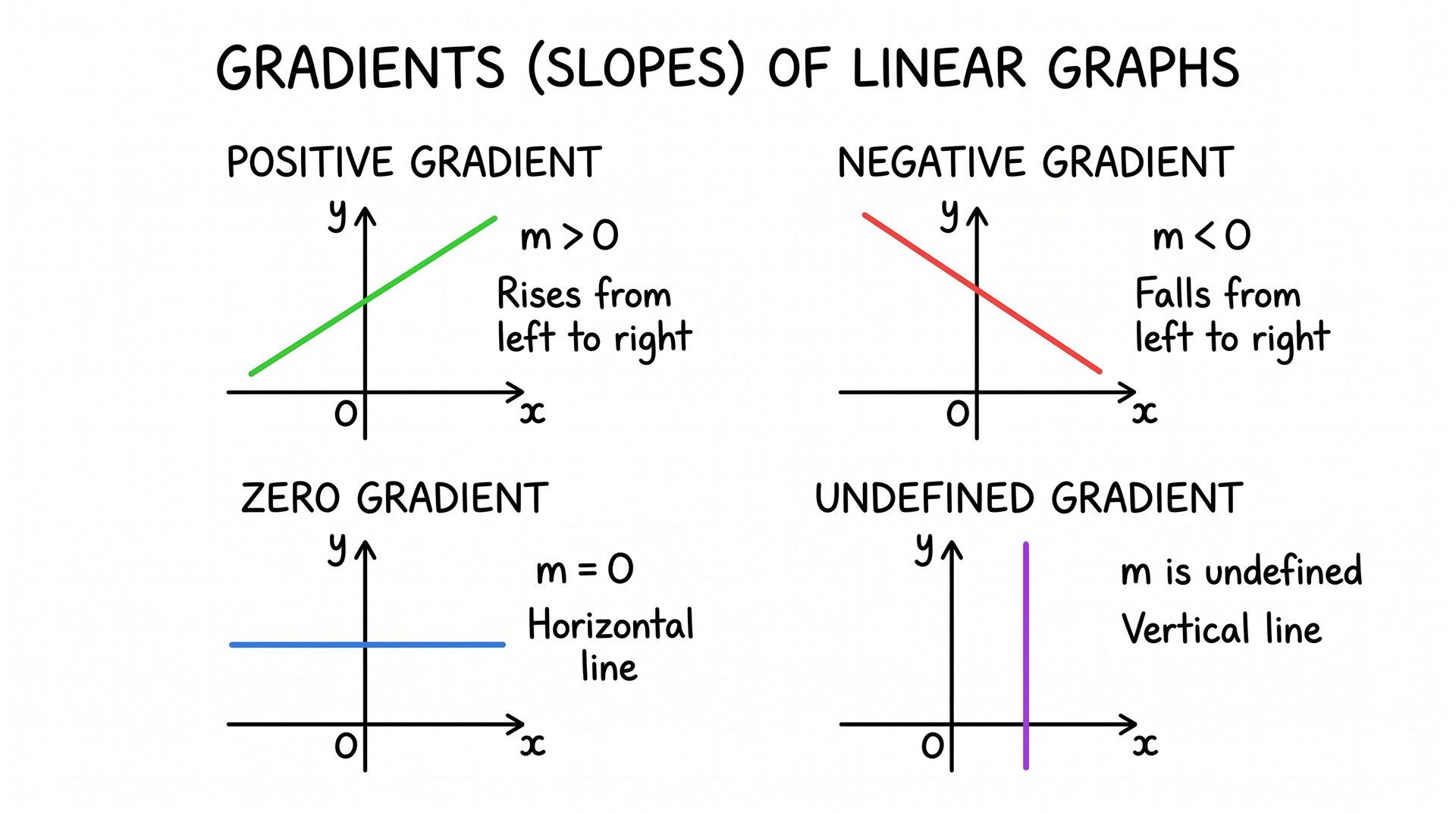
The Gradient (m): Steepness and Direction
The gradient (m) measures the rate at which the line rises or falls per unit increase in x.
The Intercepts: Crossing the Axes
Every oblique linear function crosses both Cartesian axes:
The y-Intercept
The point where the line crosses the vertical axis (x = 0):
In real-world modeling, c frequently represents the initial value or fixed starting cost before any change occurs.
The x-Intercept
The point where the line crosses the horizontal axis (y = 0):
In real-world applications, this represents the break-even point or the threshold where the quantity reaches zero.
Worked Examples
Worked Example 1: Calculating Gradient and Forming y = mx + c
A straight line passes through the points A(-3, 11) and B(5, -5).
(a) Calculate the gradient of the line.
(b) Determine the equation of the line in the form y = mx + c.
(c) State the coordinates of the x-intercept.
Step 1: Calculate the gradient (m)
Step 2: Find the y-intercept (c)
Substitute m = -2 and the coordinates of point B(5, -5) into y = mx + c:
The equation of the line is:
Step 3: Calculate the x-intercept
Set y = 0:
The x-intercept is (2.5, 0).
Worked Example 2: Rearranging from General Form ax + by + c = 0
A line L has the equation 4x - 6y + 15 = 0
(a) Express the equation in the form y = mx + c
(b) State the gradient and the coordinates of the y-intercept.
Step 1: Isolate the y-term
Step 2: Divide every term by the coefficient of y (6)
Step 3: Simplify all fractions to lowest terms
Step 4: Identify parameters
- Gradient:
- y-intercept: or
Practice Questions & Solutions
A line passes through the coordinates A(-2, -7) and B(3, 8).
(a) Calculate the gradient of the line.
(b) Find the equation of the line in the form y = mx + c
(c) Determine the exact coordinates of the point where the line crosses the x-axis.
(a)
Calculate the gradient m using the coordinates A(-2, -7) and B(3, 8):

(b)
Use point-gradient form with point B(3, 8):




(c)
To find the x-intercept, set y = 0:

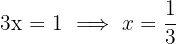
Coordinates of the x-intercept:
 .
.
Line  has the equation
  .
.
Line  is parallel to and passes through the point (-5, 4).
Find the equation of in the form  , where
  and a > 0.
Step 1: Determine the gradient of
Rearrange into  form:
form:

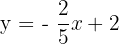
The gradient of is  .
.
Step 2: Form the equation of parallel line
Since  ,
,  .
.
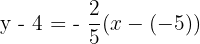
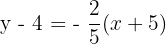
Using point  :
:

Step 3: Convert to general form
Multiply every term by  to eliminate the fraction:


Rearrange all terms to the left side:
A straight road is modeled by the line  .
.
A pedestrian pathway connects perpendicular to this road, meeting it at the point where the road crosses the y-axis.
(a) Find the coordinates of the road's y-intercept.
(b) Find the gradient of the perpendicular pathway.
(c) Write down the equation of the pathway in the form .
(a)
Find the y-intercept of the road by setting x = 0:


The intersection point is (0, 2)
(b)
Rearrange the road's equation to find its gradient  :
:

The gradient of the road is  .
.
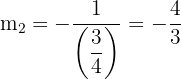
The gradient of the perpendicular pathway  is the negative reciprocal:
(c)
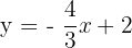
The pathway passes through (0, 2) with gradient  :
:
Summarise with AI:
Did you like this article? Rate it!

 Loading...
I get it somehow, there are others who are unfamiliar and I have a hard time with it but it’s okay that I get it.
Thanks for sharing your thoughts! It’s completely normal to find some parts unfamiliar or more difficult than others. The important thing is that you’re making progress and understanding more as you practise. Keep going! 😊
At least I understood some of it, but there are others that I’m confused about and have a hard time understanding, but I get it.
Thanks for sharing! It’s great that you’ve understood some of it already. Don’t worry if a few parts are still confusing — keep practising and take your time with the trickier sections. You’ll get there! 😊
The lesson was a little difficult for me, especially the word problems, but the examples helped me understand it better.
Thanks for your feedback! Word problems can definitely be tricky, so we’re glad the examples helped make the lesson clearer. Keep practising — it gets easier with time! 😊
Thankyouuu po