In this article, we will employ Spearman’s rank correlation and Pearson’s linear correlation to assess the relationships between two variables. This will include how biotic and abiotic factors affect the distribution and abundance of species. We will also use Simpson’s index of diversity (D) to compute the biodiversity of an area, and state the significance of different values of D.


Correlation
Various trends should be observed while recording the abundance and distribution of species in a specific area. Sometimes, the data shows the correlation between the variables. We can define correlation as:
The relationship or association between variables is referred to as correlation
Difference Between Causation and Correlation
Remember that correlation and causation are two different concepts. A correlation does not always indicate a causative relationship between the two variables. On the other hand, causation takes place when one variable influences or get influenced by another variable.
Correlation Between Species
Correlation can occur between the species. For instance, two species are always found close to each other. There can be a correlation between species and an abiotic factor. For instance, if a specific plant species are found in an area that contains a certain soil Ph. We can employ scatter graphs and various statistical tests to analyze the visible correlation between the variables.
Correlation Between Two Variables
To comprehend the correlation between two variables, we can plot the data points of both variables on the scatter graph.
- Correlation coefficient: The strength of the relationship between two variables is depicted by a correlation coefficient (r).
- Perfect correlation: If all the data points fall on a straight line and the correlation coefficient is 1 or -1, then we say that there is a perfect correlation between the two variables.
- Positive or negative correlation: There can be a positive or negative correlation between the two variables.
- Positive correlation: Suppose there are two variables A and B. There is a positive correlation between these two variables if variable A increases as variable B increases
- Negative correlation: There is a negative correlation between two variables A and B, if variable A increases, the variable B decreases
- No correlation: The correlation coefficient will be zero if there is no correlation between the variables
We can compute the correlation coefficient (r) to determine whether there is a linear relationship between variables. It can also be used to determine the strength of the relationship between the two variables.
Pearson Linear Correlation
We can define Pearson’s linear correlation as:
A statistical test that tells whether there is a linear correlation between two variables or not is known as Pearson’s linear correlation
For this test, the data should be:
- Quantitative
- Exhibit normal distribution
Procedure
Follow these steps to carry out this test:
- Step 1: Make a scatter graph of the data obtained and determine if there is a linear relationship between the variables.
- Step 2: Write the null hypothesis
- Step 3: Use the equation below to calculate the Pearson’s correlation coefficient r:
In the above equation:
- r represents the correlation coefficient
- x depicts the number of species A
- y represents the number of species B
- n represents the number of readings
 represents the standard deviation of species A
 represents the standard deviation of species B
 represents the number of species A
 represents the number of species B
If the correlation coefficient comes out to be 1 or -1, then we can say that there is a strong linear correlation between the two variables. We can also say that the null hypothesis can be rejected.
Spearman's Rank Correlation
Pearson’s linear correlation should not be used under the following two conditions:
- There is no visible relationship between the two variables
- The data does not exhibit a normal distribution
Spearman’s rank calculation tells us if there is a correlation between the variables that do not exhibit a normal distribution.
Procedure to Use this Test
Follow the steps below to use this test:
- Step 1: Create a scatter graph and determine the possible linear correlation
- Step 2: Write the null hypothesis
- Step 3: Use the equation below to calculate the Spearman’s rank correlation coefficient r:
In the above equation:
-
 represents the spearman’s rank coefficient
- D depicts the difference in rank
- n represents the number of samples
- Step 4: See the table that relates critical values of to probability levels
We can reject the null hypothesis if the value computed for Spearman’s rank is more than the critical value for the number of samples in the data (n) at the probability level (p) 0.05. It implies that a correlation exists between the two variables.
Solved Example
Suppose a student conducted an experiment by using quadrats to measure the abundance of various species of plants in a neglected allotment. The purpose is to observe any correlation between the abundance of species C and D. When they observed the data and created a scatter graph, they observed a correlation. Your task is to find the possible correlation by employing Spearman’s rank correlation coefficient.
The decision to employ Spearman’s rank correlation coefficient was because the data was not normally distributed. The null hypothesis is:
There is no correlation between the abundance of species A and species B.
n = 10 because there are 10 quadrat samples
Because the data was not normally distributed, therefore they decided to employ Spearman’s rank correlation coefficient.
Procedure
Follow these steps to calculate Spearman’s rank coefficient.
- Step 1: First, rank each data set
- Step 2: Calculate the rank difference between the two species, D
- Step 3: In this step, square the rank difference found in step 2,

- Step 4: In this step, substitute the suitable numbers into the equation
- Step 5: See the table that relates values to probability. Look for the probability level of 0.05 with n = 10
Critical value of at n = 10 = 0.65
Because  = 0.964, hence it is greater than the critical value of 0,65. Thus, we can reject the null hypothesis because there is a real positive correlation between the abundance of species A and species B.
Simpson’s Index
After recording the abundance of various species in an area, the results should be used to compute the diversity of species or biodiversity for that area. Species diversity observes the number of various species in an area along with the evenness of abundance across different species. Simpson’s index of diversity (D) can be employed to quantify the biodiversity of an area.
The formula is given below:
Here:
-
-
- n represents the total number of organisms for a single species
- N depicts the total number of organisms for all species
-
Follow these steps to compute the Simpson’s Index:
- Step 1: Calculate
 for each species
 - Step 2: Square each of these values
- Step 3: In this step, add the values obtained in step 2 and subtract the total from 1
The possible D values are significant because the value of D lies between 0 and 1.
- Values close to 1 show high levels of biodiversity
- Values close to 0 show low levels of biodiversity
Solved Example
Samples of various species of insect in a back garden were accumulated using sweep nets and identification keys. To compute the Simpson’s index use the data below.
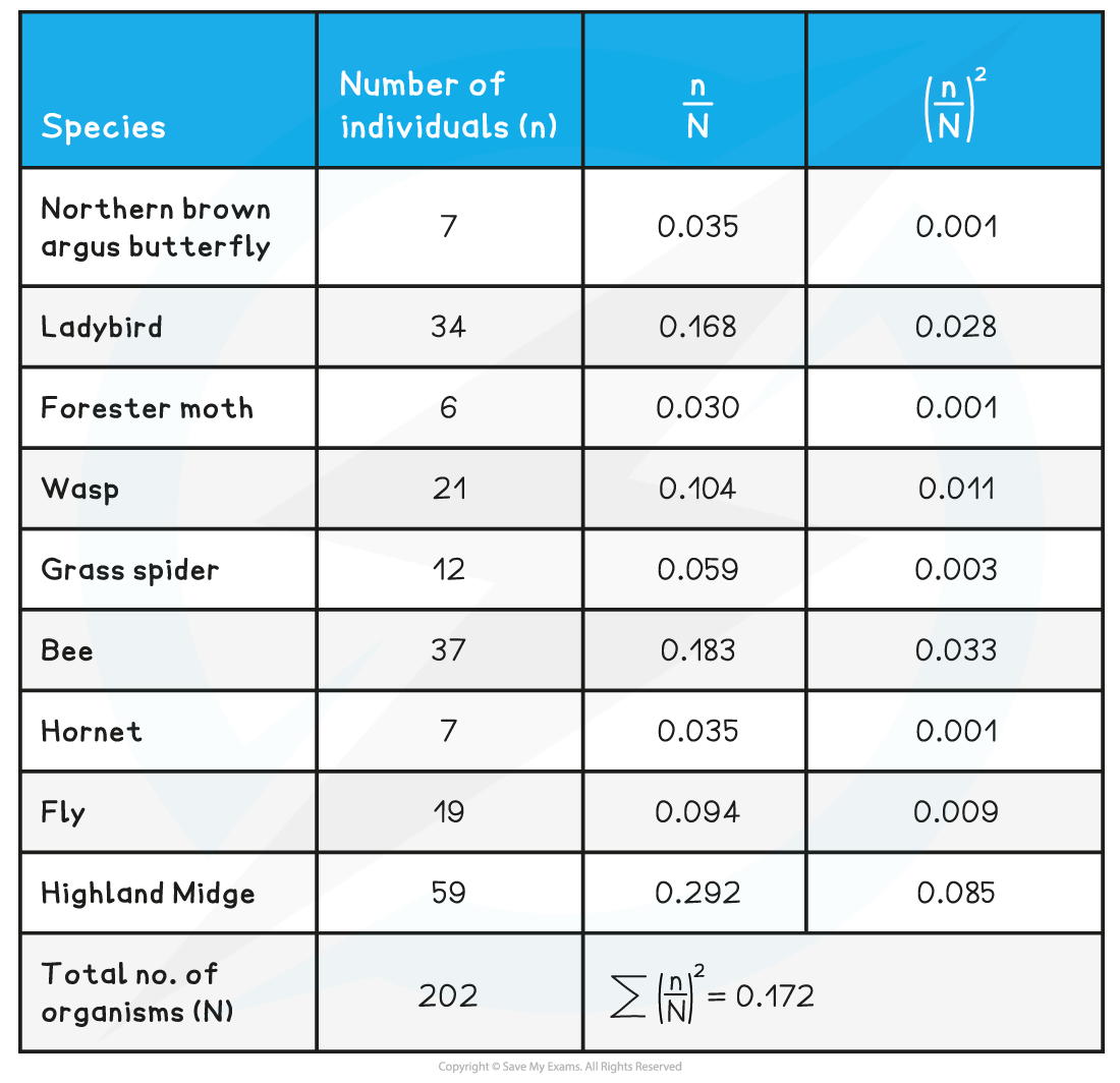
D = 1 – 0.172 = 0.828
Because the value of D is quite closer to 1 as compared to 0, hence we can say that it is a relatively high value for biodiversity.
Summarise with AI:
Did you like this article? Rate it!


